Robotic Manipulators
Lecture 1: Introduction to the Course
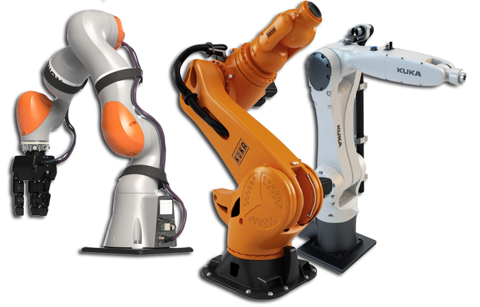
Topics Covered
- Initial information
- Course scope
- Applications
- Basic concepts
- Course syllabus
- The UAIBot simulator
- Practical assignment
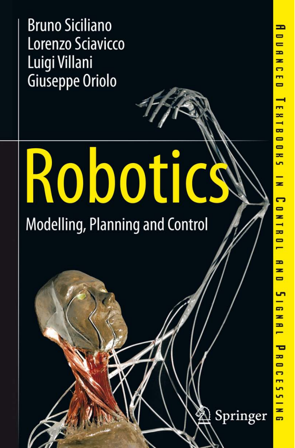
Textbook
Robotics, Modelling, Planning and Control
Bruno Siciliano
Lorenzo Sciavicco
Luigi Villani
Giuseppe Oriolo
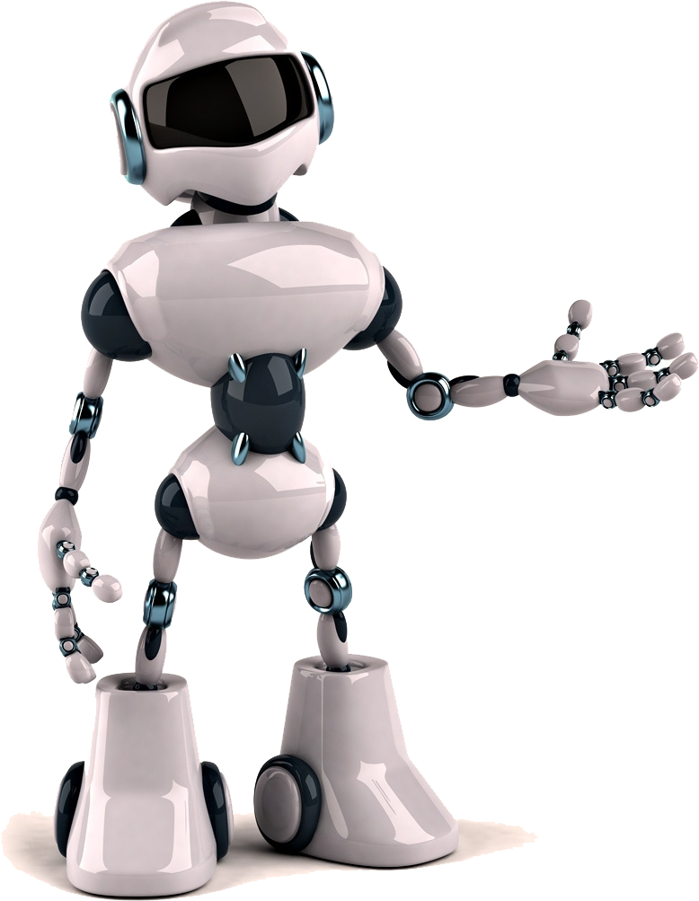
Course Scope
Classification by type of movement:

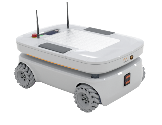
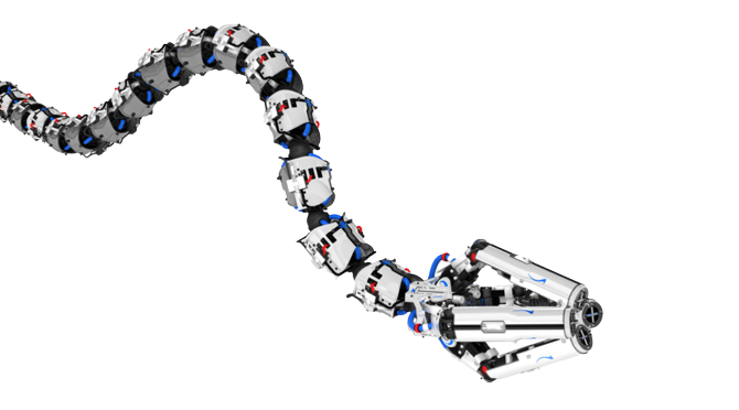
Course Scope
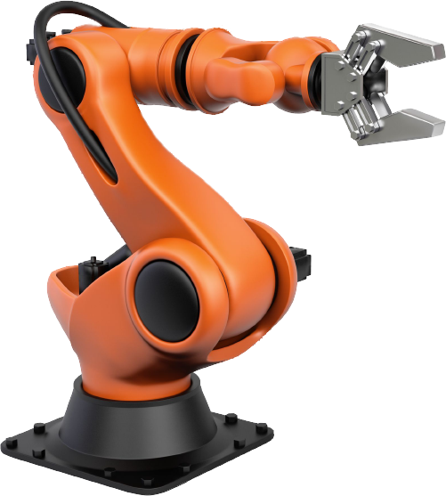
In this course, our focus is on manipulator robots:
- Fixed base, “welded” to the floor.
- A set of rigid links connected by joints that move the robot.
- A set of motors move the joints.
- An end-effector interacts with the environment.
However, most of the concepts presented in this course apply to robotics in general.
We are interested in the mathematical modeling of these robots and in their control.

Applications

Applications
Robotic Welding
Applications
Automotive Sector
Applications
Pharmaceutical Sector
Applications
Surgeries
Basic Concepts

Basic Concepts
Types of Joints
There are others (spherical, cylindrical), but these are the basics.
Basic Concepts
Degrees of Freedom (DoF)
Basic Concepts
Degrees of Freedom (DoF)
Constraints can reduce the degrees of freedom.
The robot shown, which normally has 6 degrees of freedom, is constrained so its end-effector is
“attached” to the ground.
Four constraints:
- Fixed z-position (height) at the end-effector;
- Fixed rotation in x at the end-effector;
- Fixed rotation in y at the end-effector;
- Fixed rotation in z at the end-effector.
6 joints - 4 constraints = 2 degrees of freedom.
Basic Concepts
Workspace

Basic Concepts
Classic Robot Configurations
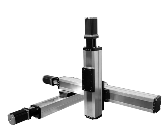
Cartesian: three linear joints.
The three joints are orthogonal.
The workspace is a box.
Very simple to model/control.
It is not possible to control the orientation of the end-effector.
Widely used in 3D printing, for example.
Basic Concepts
Classic Robot Configurations
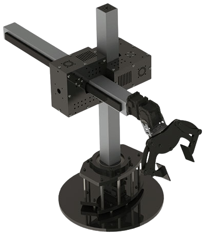
Cylindrical: two linear joints and one revolute joint.
Good speed and accuracy in control (roughly speaking: revolute joints are faster than linear).
The workspace is a cylinder.
Used in pick-and-place tasks.
Basic Concepts
Classic Robot Configurations
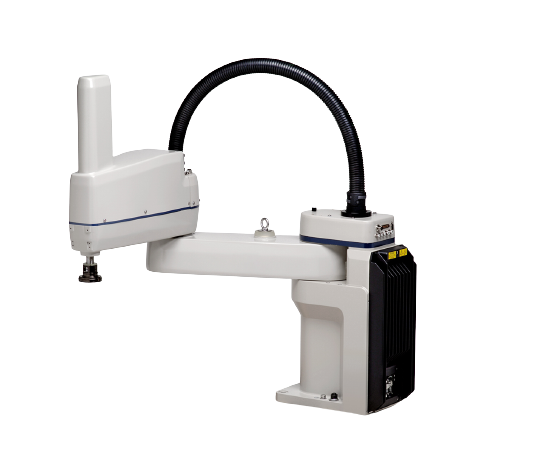
SCARA (Selective Compliance Articulated Robot Arm): two revolute joints and
one linear joint.
Very fast (faster than cylindrical).
The workspace is a cylinder.
Compliance is the ability of a system to be flexible and adapt to the force
acting on it. SCARA robots have slight compliance in the x and y axes (but not in z), allowing
their revolute joints to move slightly when under force. It is, in a way, the opposite of rigidity.
Used in tasks that require applying force (e.g., inserting one part into another).
Course Syllabus

Course Syllabus
- Spatial description
- Direct and inverse kinematics
- Differential kinematics
- Kinematic control
- System dynamics
- Dynamic control
- ROS

Course Syllabus
Spatial Description
Goal: describe the robot’s motion.
Our manipulators are composed of rigid bodies (the links) connected
sequentially. Describing their motion means describing the robot’s motion.
Rigid bodies are objects that cannot be deformed, broken, or fused together.
How to describe the motion of these objects?
In high school physics, we learned how to describe the motion of a particle in 3D space. For that, given a reference frame
\(\mathcal{F}_0\), we provide at every time instant \(t\) the coordinates \(x(t)\),
\(y(t)\), and \(z(t)\) of the particle in \(\mathcal{F}_0\).
Note that for a particle, rotation is irrelevant (its dimensions are negligible, i.e. it
has no volume).
The motion of rigid bodies can be described by “attaching” a reference frame to the object
and describing the (translation + rotation) of that frame. We will need to provide more
info than just \(x(t)\), \(y(t)\), and \(z(t)\).
Position + orientation = pose of the object.
Course Syllabus
Direct and Inverse Kinematics
Goal: describe the motion of the robot’s end-effector, which is a
rigid body.
Since the only motion the robot has comes from its joints, there must
be a mathematical mapping between the current position of the joints (time-varying
variables) and the robot’s structural parameters (fixed) in the mathematical description
of the end-effector’s pose with respect to a reference frame
\(\mathcal{F}_0\).
Let \(q\) be a vector with the position of all the joints, and \(T\) be the description of
the end-effector in \(\mathcal{F}_0\). Then there must be a mathematical function \(f\)
such that \(T = f(q)\).
The function \(f\) is called the direct kinematics of the
end-effector.
It allows us to calculate where the end-effector is, based on the joint positions in the
vector \(q\).
The inverse kinematics solves the opposite problem: given a pose
\(T\), what is the value of the joints \(q\) such that \(T = f(q)\)?
Both problems are important because we will control the joint positions \(q\) aiming for
the end-effector to reach a certain pose \(T\). The two functions describe how these two
quantities relate in both directions.

Course Syllabus
Differential Kinematics
Goal: describe the motion of the robot’s end-effector, which is a
rigid body.
Direct and inverse kinematics map positions (of the joints) to “positions” of the end-effector (for a rigid body, “position”
should be understood as “pose”).
In control, this is not enough. We also need to relate velocities.
A rigid body has two velocity vectors, both 3-dimensional:
- Linear velocity, \(v\)
- Angular velocity, \(\omega\)
The goal of differential kinematics is: given that at a time instant
the joint positions are \(q\) and the instantaneous velocity of the
joints is \(\dot{q}\), determine \(v\) and \(\omega\) at that same instant.
Hence there are functions \(g_v\) and \(g_{\omega}\) such that \(v = g_v(q,\dot{q})\) and
\(\omega = g_{\omega}(q,\dot{q})\).

Course Syllabus
Kinematic Control
Goal: control the robot’s joints so the end-effector reaches a
desired pose.
Here we will make a (very reasonable) assumption about the robot: it has a programming
interface allowing us to send, every control cycle, a desired joint velocity for each
joint, here called \(u\).
We assume it follows this sent command perfectly. Therefore, we consider a control system in which the manipulated variable
\(u\) is the desired joint velocity, and the process variable \(q\) is the joint position.
The model relating the two is $$\dot{q} = u.$$
Thus, given a desired end-effector pose \(T_{des}\), we want to design a controller (algorithm) using the current joint position \(q\)
(closed-loop) that ensures the end-effector, from any initial pose, will reach the
desired pose.
This is called kinematic control because it abstracts the system’s dynamics, i.e., the forces/torques acting on the robot
and the masses/inertia involved.
The controller uses direct kinematics and differential kinematics to compute the control
action.
Generally, the control is nonlinear, because the function \(h(q)\) is
typically nonlinear.


Course Syllabus
System Dynamics
Goal: control the robot’s joints to reach a desired end-effector
pose, but now without assuming the robot has a high-level velocity control interface.
We will act directly on the torque of the motors driving the
joints.
Hence we are no longer talking about kinematics, but dynamics, since forces/torques acting on the robot and the masses/
inertias of its rigid bodies become relevant.
We thus need to write the robot’s dynamic equations, that is, a
differential equation relating how the position and velocity of all its particles
evolve, given the system parameters (such as masses and inertias) and the forces
(which can be time-varying).
Since the motion of all particles in the robot depends only on the
motion of the joints (because they are rigid bodies), and assuming the only force acting
on the system is the torque at each motor, \(\tau\), we want to
find the differential equation $$\ddot{q} = F(q,\dot{q},\tau)$$ that
relates these variables.
Applying Newton’s Laws to each (infinite) particle that makes up the
robot is not feasible. Fortunately, there are various ways to overcome this problem...

Course Syllabus
Dynamic Control
Goal: control the robot’s joints to reach a desired end-effector
pose, but now without assuming the robot has a high-level velocity control interface.
We will act directly on the torque of the motors driving the
joints.
Using the robot’s dynamic model, \(\ddot{q} = F(q,\dot{q})\), we can design a control law
$$\tau = h(q, \dot{q})$$
using the position and velocity of the joints to reach a desired pose \(T_{des}\).
Here we assume that the only forces acting on the robot come from the motors, and thus are
completely controllable. Therefore, there is no external force (like contact with the
environment).
One way to design dynamic control is to start from kinematic control.
Generally, the control is nonlinear because the function
\(h(q,\dot{q})\) is usually nonlinear.
Q: What is the advantage of dynamic control over kinematic control?
A: With it, we can implement certain tasks that wouldn’t be
possible with kinematic control alone. In particular, it forms the basis for force control (not covered in this course), where external forces
on the robot are considered. Such control is needed for tasks in which the robot must
exert a controlled force on the environment.


Course Syllabus
ROS
ROS (Robotic Operating System): widely used software in academia and industry
to handle communication between control code (C++, Python, etc.) and robots;
It allows code reuse on different robots because it abstracts away specific communication details
(i.e., it talks with each robot’s drivers).
It is similar to the OPC concept in automation.
We will see introductory notions of this software in this course.

UAIBot
UAIBot is an open-source robotics simulator.
The code is done in Python, and the simulation visualization can be done right in the browser
without installing any additional software.
The generated animations are .html files that can be viewed in any browser.
We will use this simulator in the course.
Project GitHub:
https://github.com/UAIbot/UAIbotPy.

UAIBot
Installation
There are several ways to use/install UAIBot:
Using an IDE (like PyCharm), type in the terminal:
>>pip install uaibot
After installation, test by running a simulation already included in the package. For that,
run the following Python code:
import uaibot as ub

sim = ub.Demo.control_demo_1()
sim.save('C:\\','teste_controle_1')

UAIBot
GOOGLE COLAB
If you do not want to use a desktop IDE, you can use the online collaborative platform Google Colab,
keeping everything in the browser.
In Google Colab, run the command to install UAIBot:
!pip install uaibot
Note that this needs to be done every time you restart Google Colab.
In Google Colab, there is no need to use the “save” function. Simulations are shown
directly in the browser. Running the code below will automatically display the
simulation:
import uaibot as ub

sim = ub.Demo.control_demo_1()

UAIBot
DEMONSTRATION
UAIBot
DEMONSTRATION
UAIBot
DEMONSTRATION
Practical Assignment

Practical Assignment
For the final project of this course, you must implement a robotics application in the UAIBot
simulator.
You must choose a suitable robot for the application. The implementation must consider practical
limitations of the robot such as joint limits, motor velocity, and torque,
etc.
More information (dates, instructions, etc.) coming soon.